Efficient Interpolation with Caching

Interpolation is a common method to perform computationally expensive tasks more cheaply. However, widely available methods generally assume that one will generate a single interpolant designed to be evaluated at many points.

When performing a Bayesian analysis with a stochastic sampler however, one sometimes has to evaluate many interpolants (representing the parameterized model) at the same set of points (the data) with the same knot points.

Evaluating interpolants typically requires two stages:

1. finding the closest knot of the interpolant to the new point and the distance from that knot.
2. evaluating the interpolant at that point.

When we have identical knots and evaluation points but different functions being approximated the first of these stages is done many times unnecessarily. This can be made more efficient by caching the locations of the evaluation points leaving just the evaluation of the interpolation coefficients to be done at each iteration.

A further advantage of this, is that it allows trivially parallising the interpolation using cupy.

This package implements this caching for nearest neighbour, linear, and cubic interpolation.

Installation

Currently this is only installable by downloading the source and installing locally.

$ git clone git@github.com:ColmTalbot/cached_interpolation.git
$ cd cached_interpolation
$ pip install .

Demonstration

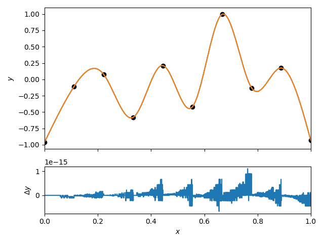
We can compare the interpolation to the scipy.interpolate.CubicpSpline implementation.

import numpy as np
import matplotlib.pyplot as plt
from scipy.interpolate import CubicSpline

from cached_interpolate import CachingInterpolant

x_nodes = np.linspace(0, 1, 10)
y_nodes = np.random.uniform(-1, 1, 10)
evaluation_points = np.sort(np.random.uniform(0, 1, 10000))

interpolant = CachingInterpolant(x=x_nodes, y=y_nodes, kind="cubic")
sp_interpolant = CubicSpline(x=x_nodes, y=y_nodes, bc_type="natural")

figure, axes = plt.subplots(nrows=2, gridspec_kw={'height_ratios': [3, 1]}, sharex=True)
axes[0].plot(evaluation_points, interpolant(evaluation_points))
axes[0].plot(evaluation_points, sp_interpolant(evaluation_points))
axes[0].scatter(x_nodes, y_nodes, color="k")
axes[1].plot(evaluation_points, interpolant(evaluation_points) - sp_interpolant(evaluation_points))
axes[0].set_ylabel("$y$")
axes[1].set_xlabel("$x$")
axes[1].set_ylabel("$\\Delta y$")
axes[1].set_xlim(0, 1)
plt.tight_layout()
plt.show()
plt.close(figure)

I note here that we use the “natural” boundary condition. This means that first and second derivatives of the spline vanish at the endpoints. This is different from the default “not-a-knot” boundary condition used in scipy.

We can now evaluate this interpolant in a loop to demonstrate the performance of the caching. At every iteration we change the function being interpolated by randomly setting the y argument. Before the loop, we add an initial call to set up the cache as this will be much slower than the following iterations.

import time

import numpy as np
from scipy.interpolate import CubicSpline

from cached_interpolate import CachingInterpolant

x_nodes = np.linspace(0, 1, 10)
y_nodes = np.random.uniform(-1, 1, 10)
evaluation_points = np.random.uniform(0, 1, 10000)

interpolant = CachingInterpolant(x=x_nodes, y=y_nodes, kind="cubic")
sp_interpolant = CubicSpline(x=x_nodes, y=y_nodes, bc_type="natural")

interpolant(x=evaluation_points, y=y_nodes)

n_iterations = 1000

start = time.time()
for _ in range(n_iterations):
    y_nodes = np.random.uniform(-1, 1, 10)
    interpolant(x=evaluation_points, y=np.random.uniform(-1, 1, 10))
stop = time.time()
print(f"Cached time = {(stop - start):.3f}s for {n_iterations} iterations.")

start = time.time()
for _ in range(n_iterations):
    y_nodes = np.random.uniform(-1, 1, 10)
    CubicSpline(x=x_nodes, y=y_nodes, bc_type="natural")(evaluation_points)
stop = time.time()
print(f"Scipy time = {(stop - start):.3f}s for {n_iterations} iterations.")

Cached time = 0.187s for 1000 iterations.
Scipy time = 0.450s for 1000 iterations.

We’ve gained a factor of ~2.5 over the scipy version without caching. If this is the dominant cost in a simulation that takes a week to run, this is a big improvement.

If we need to evaluate for a new set of points, we have to tell the interpolant to reset the cache. There are two ways to do this:

• create a new interpolant, this will require reevaluating the interplation coefficients.
• disable the evaluation point caching.

import numpy as np
from scipy.interpolant import CubicSpline

from cached_interpolate import CachingInterpolant

x_nodes = np.linspace(0, 1, 10)
y_nodes = np.random.uniform(-1, 1, 10)
evaluation_points = np.random.uniform(0, 1, 10000)

interpolant = CachingInterpolant(x=x_nodes, y=y_nodes, kind="cubic")
interpolated_values = interpolant(evaluation_points)

new_evaluation_points = np.random.uniform(0, 1, 1000)
interpolant(x=new_evaluation_points, use_cache=False)

Using the code in this way is much slower than scipy and so not practically very useful.

If you have access to an Nvidia GPU and are evaluating the spline at ~ O(10^5) or more points you may want to switch to the cupy backend. This uses cupy just for the evaluation stage, not for computing the interpolation coefficients.

import cupy as cp
import numpy as np

from cached_interpolate import CachingInterpolant

x_nodes = np.linspace(0, 1, 10)
y_nodes = np.random.uniform(-1, 1, 10)
evaluation_points = np.random.uniform(0, 1, 10000)
evaluation_points = cp.asarray(evaluation_points)

interpolant = CachingInterpolant(x=x_nodes, y=y_nodes, backend=cp)
interpolated_values = interpolant(evaluation_points)

We can now repeat our timing test. To make the use of a GPU more realistic we’ll increase the number of evaluation points.

import time

import cupy as cp
import numpy as np
from scipy.interpolate import CubicSpline

from cached_interpolate import CachingInterpolant

x_nodes = np.linspace(0, 1, 10)
y_nodes = np.random.uniform(-1, 1, 10)
evaluation_points = np.random.uniform(0, 1, 100000)
cp_evaluation_points = cp.asarray(evaluation_points)

interpolant = CachingInterpolant(x=x_nodes, y=y_nodes, kind="cubic")
cp_interpolant = CachingInterpolant(x=x_nodes, y=y_nodes, kind="cubic", backend=cp)
sp_interpolant = CubicSpline(x=x_nodes, y=y_nodes, bc_type="natural")

interpolant(x=evaluation_points)
cp_interpolant(x=cp_evaluation_points)

n_iterations = 1000

start = time.time()
for _ in range(n_iterations):
    y_nodes = np.random.uniform(-1, 1, 10)
    interpolant(x=evaluation_points, y=np.random.uniform(-1, 1, 10))
stop = time.time()
print(f"CPU cached time = {(stop - start):.3f}s for {n_iterations} iterations.")

start = time.time()
for _ in range(n_iterations):
    y_nodes = np.random.uniform(-1, 1, 10)
    CubicSpline(x=x_nodes, y=y_nodes, bc_type="natural")(evaluation_points)
stop = time.time()
print(f"Scipy time = {(stop - start):.3f}s for {n_iterations} iterations.")

start = time.time()
for _ in range(n_iterations):
    y_nodes = np.random.uniform(-1, 1, 10)
    cp_interpolant(x=cp_evaluation_points, y=np.random.uniform(-1, 1, 10))
stop = time.time()
print(f"GPU cached time = {(stop - start):.3f}s for {n_iterations} iterations.")

CPU cached time = 3.367s for 1000 iterations.
Scipy time = 4.213s for 1000 iterations.
GPU cached time = 0.212s for 1000 iterations.

While there are likely more optimizations that can be made and improved flexibility in the implementation, we can see that the GPU version is well over an order of magnitude faster than either of the CPU versions.

If you have any comments/questions feel free to contact me through the issue tracker or a pull request on Github.