Constrained Priors in Bilby

In version 0.4.3 we introduced a new prior class: Constraint. This allows cuts to be specified in the prior space.

Simple example

For example imagine we wanted to sample from uniform distributions in two parameters x and y but we want to enforce that x >= y. In bilby we do this by introducing a dummy parameter z = x - y and enforce that z > 0.

The first thing we have to do is define a function which generates z from x and y.

Note:

• this takes in a dictionary, or any similar object.
• returns a modified version of that dictionary including our dummy parameter.

def convert_x_y_to_z(parameters):
    """
    Function to convert between sampled parameters and constraint parameter.

    Parameters
    ----------
    parameters: dict
        Dictionary containing sampled parameter values, 'x', 'y'.

    Returns
    -------
    dict: Dictionary with constraint parameter 'z' added.
    """
    parameters['z'] = parameters['x'] - parameters['y']
    return parameters

Now we have our conversion function we need to create our prior.

Note:

• when creating our PriorDict we specify our conversion function.
• we define our priors for x, y, and z.
• the x and y priors can be any prior class available in bilby.
• the z prior is a Constraint.

from bilby.core.prior import PriorDict, Uniform, Constraint

priors = PriorDict(conversion_function=convert_x_y_to_z)
priors['x'] = Uniform(minimum=0, maximum=10)
priors['y'] = Uniform(minimum=0, maximum=10)
priors['z'] = Constraint(minimum=0, maximum=10)

As a quick check we’ll sample from this distribution and plot the samples.

import matplotlib.pyplot as plt

samples = priors.sample(1000000)
plt.hist2d(samples['x'], samples['y'], bins=100, cmap='Blues')
plt.xlabel('$x$')
plt.ylabel('$y$')
plt.tight_layout()
plt.show()
plt.close()

{: width=“100%”}

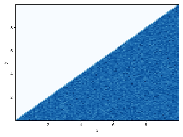
Success! All of our samples have x > y.

Gravitational wave example

Now let’s try a a quick example for gravitational-wave data analysis. There are defaults set up within bilby for analysis binary black hole and binary neutron star coalescences.

• For binary black holes, the BBHPriorDict has a built-in conversion function which will allow arbitrary constraints to be placed on mass parameters.
• For binary neutron stars, constraints can also be placed on the tidal parameters with the BNSPriorDict.

An example of using constrained priors for a binary black hole system is shown below. In this example we demand that the black hole labelled 1 is more massive.

It is most intuitive to use priors which are uniform in component masses.

However, the most well measured parameter for all binary mergers except the most massive binary black hole systems is the “chirp mass”. By imposing cuts in chirp mass we can reduce the size of the prior space used for component masses.

Additionally, the waveform models we use are only trustworthy for certain mass ratios. We therefore want to impose cuts in the allowed mass ratios.

As an example we consider the binary black hole detection GW151226.

First we set up the BBHPriorDict and specify our priors on the component masses. Note:

• no conversion function is specified here, in this case, it defaults to a function which gets all the mass and tidal parameters bilby knows about.

from bilby.core.prior import Uniform, Constraint
from bilby.gw.prior import BBHPriorDict
priors = BBHPriorDict()
priors['mass_1'] = Uniform(minimum=3, maximum=55)
priors['mass_2'] = Uniform(minimum=3, maximum=55)

Now we need to specify our constraints.

We create two Constraint priors:

• the waveform used for the analysis is trusted for mass ratios greater than 1 / 18, and our model demands that the more massive black hole is the primary component.
• since this is a relatively low-mass event, the chirp mass is well constrained.

priors['mass_ratio'] = Constraint(minimum=1 / 18, maximum=1)
priors['chirp_mass'] = Constraint(minimum=9.5, maximum=10.5)

Again, we’ll make 2d plots of the mass and spin parameters to verify that all the samples obey the expected constraints.

import matplotlib.pyplot as plt

samples = priors.sample(1000000)
plt.hist2d(samples['mass_1'], samples['mass_2'], bins=100, cmap='Blues')
plt.xlabel('$m_1$')
plt.ylabel('$m_2$')
plt.tight_layout()
plt.show()

{: width=“100%”}

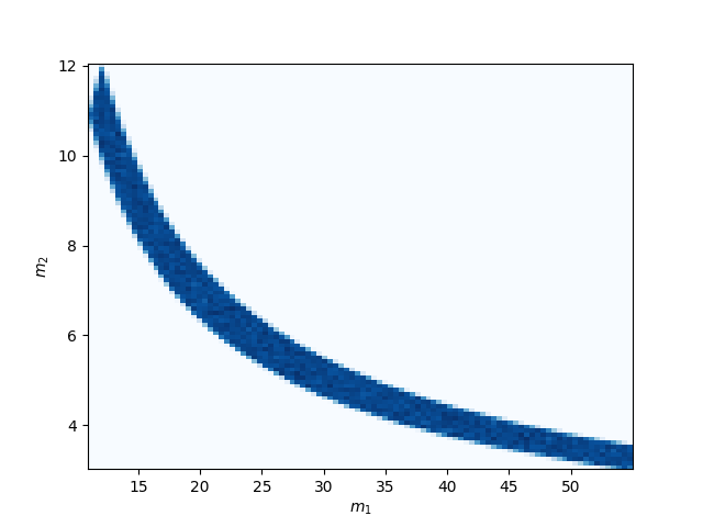
We can see that the allowed prior region is much smaller than the full component mass space.

The upper and lower limits are lines of constant chirp mass. The equal mass limit can be seen in the upper left corner.

Summary

In this post we’ve created constrained priors within bilby.

These just require a parameterisation of the cuts which are applied. Using this, arbitrary cuts can be applied to the prior used in Bayesian inference using bilby.

Note:

• when these cuts are specified the normalisation of the prior probability will not be correct. Care should therefore be taken if the normalisation of the prior needs to be known.