Compare memory calculation codes

Since the initial release of GWMemory other packages to compute the waveform have been released. For example, the sxs package has a method to compute memory.

In this notebook we compare the performance of the two packages for a test example.

NOTE: the sxs code is able to include additional memory terms beyond the dominant energy term considered here.

Thanks to Scott Field for suggesting this test.

import matplotlib as mpl
import matplotlib.pyplot as plt
import numpy as np
import gwsurrogate as gws
from gwmemory import time_domain_memory as tdm
from gwtools import sxs_memory

%matplotlib inline

/usr/share/miniconda/envs/__setup_conda/lib/python3.11/site-packages/gwtools/const.py:52: UserWarning: Wswiglal-redir-stdio:

SWIGLAL standard output/error redirection is enabled in IPython.
This may lead to performance penalties. To disable locally, use:

with lal.no_swig_redirect_standard_output_error():
    ...

To disable globally, use:

lal.swig_redirect_standard_output_error(False)

Note however that this will likely lead to error messages from
LAL functions being either misdirected or lost when called from
Jupyter notebooks.

To suppress this warning, use:

import warnings
warnings.filterwarnings("ignore", "Wswiglal-redir-stdio")
import lal

  import lal

lal.MSUN_SI != Msun
__name__ = gwsurrogate.new.spline_evaluation
__package__= gwsurrogate.new

mpl.rcParams["font.family"] = "serif"
mpl.rcParams["font.serif"] = "Computer Modern Roman"
mpl.rcParams["font.size"] = 20
mpl.rcParams["text.usetex"] = True
mpl.rcParams["grid.alpha"] = 0

Create the time domain model. We do this with the gwsurrogate package.

For this case, we will use a binary with mass ratio 8 and large aligned spins.

model = gws.LoadSurrogate("NRHybSur3dq8")
chi0 = [0, 0, 0.8]
t = np.arange(-1000, 100, 0.01)
t, h, dyn = model(8, chi0, chi0, times=t, f_low=0)

Loaded NRHybSur3dq8 model

Compute the memory with the two packages.

For comparison, we record the time taken for each code.

print("GWMemory time:")
%time h_mem, times = tdm(h_lm=h, times=t, l_max=4)
print("SXS time:")
%time h_mem_sxs, times_sxs = sxs_memory(h, t)

GWMemory time:
CPU times: user 600 ms, sys: 376 ms, total: 976 ms
Wall time: 975 ms
SXS time:
CPU times: user 5.98 s, sys: 109 ms, total: 6.09 s
Wall time: 6.07 s

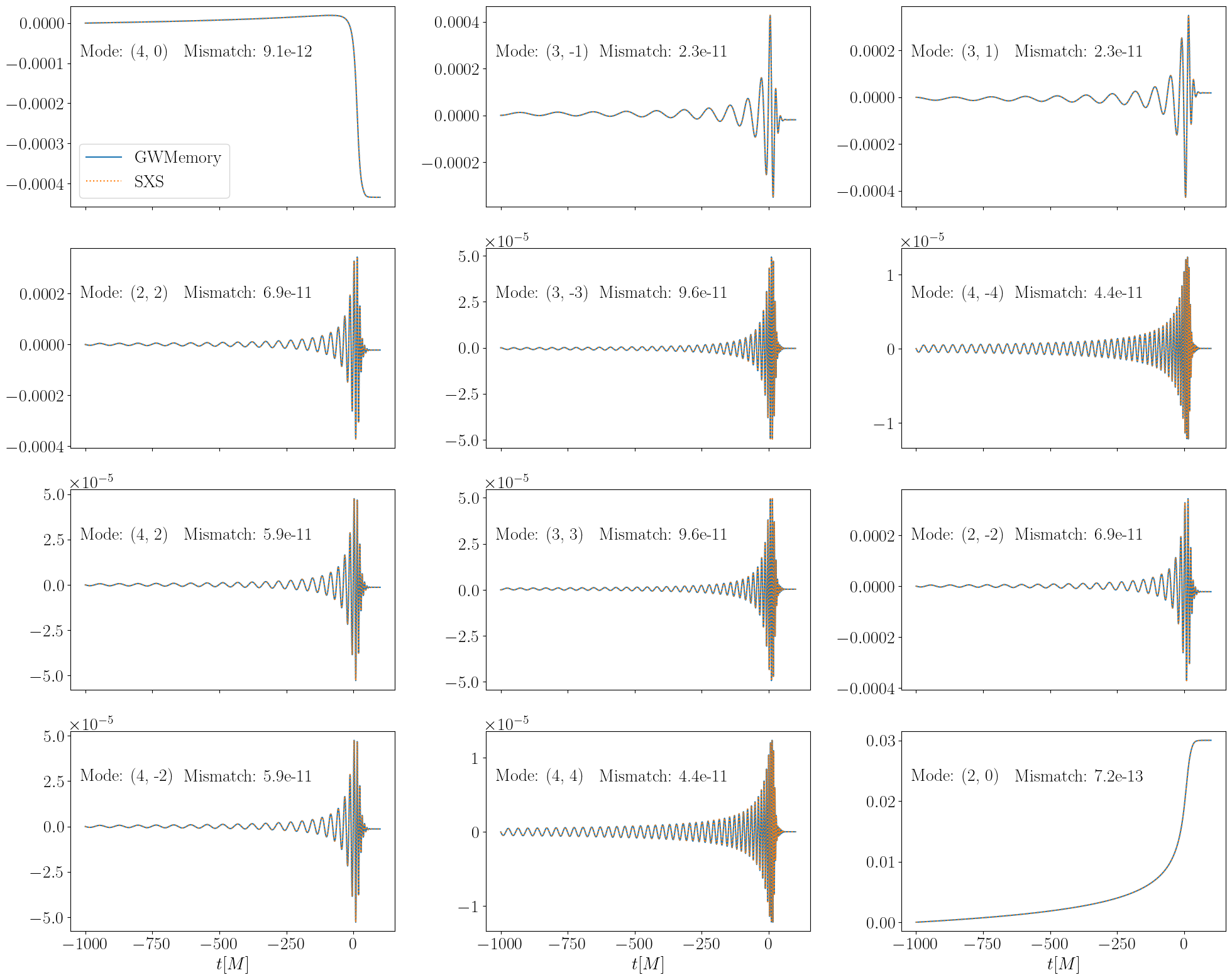
Now we plot the various memory modes along with the mismatches between the waveforms obtained with both methods.

There are some differences in strongly subdominant modes, this is likely due to numerical error accumulating for small amplitude modes. We explicitly skip these in the plotting below.

modes = set(h_mem.keys()).intersection(h_mem_sxs.keys())
for mode in modes.copy():
    if max(abs(h_mem[mode])) < 1e-15:
        modes.remove(mode)

fig, axes = plt.subplots(nrows=4, ncols=3, sharex=True, figsize=(20, 16))
for ii, mode in enumerate(modes):
    gwmem = h_mem[mode]
    sxsmem = h_mem_sxs[mode]
    overlap = (
        np.vdot(gwmem, sxsmem)
        / np.vdot(gwmem, gwmem) ** 0.5
        / np.vdot(sxsmem, sxsmem) ** 0.5
    )

    ax = axes[ii // 3, ii % 3]
    ax.plot(times, gwmem.real, label="GWMemory")
    ax.plot(times_sxs, sxsmem.real, linestyle=":", label="SXS")
    ax.annotate(f"Mode: ({mode[0]}, {mode[1]})", (0.03, 0.75), xycoords="axes fraction")
    ax.annotate(
        f"Mismatch: {1 - overlap.real:.1e}", (0.35, 0.75), xycoords="axes fraction"
    )
axes[0, 0].legend(loc="lower left")
axes[-1, 0].set_xlabel("$t [M]$")
axes[-1, 1].set_xlabel("$t [M]$")
axes[-1, 2].set_xlabel("$t [M]$")
plt.tight_layout()
plt.show()
plt.close()