Comparing the accuracy of the pade and hypergeometric integration methods in wcosmo

wcosmo supports two integration methods for evaluating integrals like \(\int \frac{dz (1 + z)^{\lambda}}{E(z)}\).

• a Pade approximation method, which is the default

• a hypergeometric method, which can be selected by setting method='analytic'

In this notebook, we compare the accuracy with respect to astropy.

The analytic and astropy method agree to machine precision and the pade method is slightly less precise. Note that only the pade method support GPU/TPU acceleration.

import wcosmo
import numpy as np
import matplotlib.pyplot as plt
from astropy.cosmology import FlatwCDM
from astropy.constants import c

# define some constants we will use throughout
Clight = c.value
z_arr = np.linspace(0.0001, 5, num=100)
H0_vals = [50, 70, 90]
Om_vals = [0.1, 0.3, 0.5, 0.9]
colors = ["blue", "orange", "purple", "green"]
w_vals = [-2, -3 / 2, -1, -1 / 2, -1 / 3, 0]

Comparisons between astropy.cosmology and wcosmo

Let’s start by determining how accurate wcosmo is for \(H_0\in [30,90] \text{km/s/kpc}\), \(\Omega_m \in [0.1,0.9]\), and \(w\in[-2,0]\).

We define two plotting functions that we will use for this whole section.

def cosmo_generator(H0, Om0, w, idx):
    if idx == 0:
        return FlatwCDM(H0=H0, Om0=Om0, w0=w)
    elif idx == 1:
        return wcosmo.FlatwCDM(H0=H0, Om0=Om0, w0=w)
    elif idx == 2:
        return wcosmo.FlatwCDM(H0=H0, Om0=Om0, w0=w, method="analytic")
    else:
        raise ValueError(f"Unknown idx {idx}")


def absolute_comparison(
    func,
    H0_arr=H0_vals,
    Om_arr=Om_vals,
    w=-1,
    colors=colors,
    linestyles=["--", "solid", ":"],
    z_arr=z_arr,
):
    fig, axes = plt.subplots(
        nrows=1, ncols=2, sharex=True, sharey=True, figsize=(10, 5)
    )
    # axis 0: vary H0
    axes[0].set_title(f"Fix $\Omega_m=0.3$, $w={w:.2f}$, vary $H_0$")
    for H0, c in zip(H0_arr, colors):
        for line, idx in zip(linestyles, range(3)):
            axes[0].plot(
                z_arr,
                cosmo_generator(H0, 0.3, w, idx).__getattribute__(func)(z_arr),
                ls=line,
                lw=3,
                c=c,
                label=f"$H_0=${H0} km/s/kpc" if idx == 0 else None,
            )
    axes[0].set_ylabel(" ".join(func.title().split("_")))

    # axis 1: vary Om0
    axes[1].set_title(f"Fix $H_0=70$, $w={w:.2f}$, vary $\Omega_m$")
    for Om, c in zip(Om_arr, colors):
        for line, idx in zip(linestyles, range(3)):
            axes[1].plot(
                z_arr,
                cosmo_generator(70, Om, w, idx).__getattribute__(func)(z_arr),
                ls=line,
                lw=3,
                c=c,
                label=f"$\Omega_m=${Om}" if idx == 0 else None,
            )

    for i in [0, 1]:
        axes[i].plot([], c="k", ls=linestyles[1], label="astropy")
        axes[i].plot([], c="k", ls=linestyles[0], lw=3, label="wcosmo - pade")
        axes[i].plot([], c="k", ls=linestyles[2], lw=3, label="wcosmo - hypergeometric")
        axes[i].legend(ncol=2)
        axes[i].set_xlabel("z")
        axes[i].set_ylim(bottom=0)
        axes[i].set_xlim(left=0)
    return fig


def fractional_comparison(
    func,
    H0_arr=H0_vals,
    Om_arr=Om_vals,
    w=-1,
    colors=colors,
    z_arr=z_arr,
    logscaley=True,
    linestyles=["--", "solid", ":"],
):
    fig, axes = plt.subplots(
        nrows=1, ncols=2, sharex=True, sharey=False, figsize=(10, 5)
    )
    # axis 0: vary H0
    axes[0].set_title(f"Fix $\Omega_m=0.3$, $w={w:.2f}$, vary $H_0$")
    for H0, c in zip(H0_arr, colors):
        ap = cosmo_generator(H0, 0.3, w, 0).__getattribute__(func)(z_arr).value
        wcos1 = cosmo_generator(H0, 0.3, w, 1).__getattribute__(func)(z_arr).value
        wcos2 = cosmo_generator(H0, 0.3, w, 2).__getattribute__(func)(z_arr).value
        fracerr_ap_wcosmo = np.abs(wcos1 - ap) / ap
        fracerr_ap_ak = np.abs(wcos2 - ap) / ap
        fracerr_ak_wcosmo = np.abs(wcos1 - wcos2) / wcos2

        axes[0].plot(
            z_arr,
            fracerr_ap_wcosmo,
            ls=linestyles[0],
            c=c,
            alpha=0.5,
            label=f"$H_0=${H0} km/s/kpc",
        )
        axes[0].plot(z_arr, fracerr_ap_ak, ls=linestyles[1], c=c, alpha=0.5)
        axes[0].plot(z_arr, fracerr_ak_wcosmo, ls=linestyles[2], c=c, alpha=0.5)
    title = " ".join(func.split("_"))
    axes[0].set_ylabel(
        "$\\frac{\\Delta \\text{%s}}{\\text{astropy %s}}$" % (title, title)
    )

    # axis 1: vary Om0
    axes[1].set_title(f"Fix $H_0=70$, $w={w:.2f}$, vary $\Omega_m$")
    for Om, c in zip(Om_arr, colors):
        ap = cosmo_generator(70, Om, w, idx=0).__getattribute__(func)(z_arr).value
        wcos1 = cosmo_generator(70, Om, w, idx=1).__getattribute__(func)(z_arr).value
        wcos2 = cosmo_generator(70, Om, w, idx=2).__getattribute__(func)(z_arr).value
        fracerr_ap_wcosmo = np.abs(wcos1 - ap) / ap
        fracerr_ap_ak = np.abs(wcos2 - ap) / ap
        fracerr_ak_wcosmo = np.abs(wcos1 - wcos2) / wcos2

        axes[1].plot(
            z_arr,
            fracerr_ap_wcosmo,
            ls=linestyles[0],
            c=c,
            alpha=0.5,
            label=f"$\Omega_m=${Om}",
        )
        axes[1].plot(z_arr, fracerr_ap_ak, ls=linestyles[1], c=c, alpha=0.5)
        axes[1].plot(z_arr, fracerr_ak_wcosmo, ls=linestyles[2], c=c, alpha=0.5)
    for i in [0, 1]:
        axes[i].legend()
        axes[i].set_xlabel("z")
        axes[i].set_xlim(left=0)
        if logscaley:
            axes[i].set_yscale("log")
        else:
            axes[i].set_ylim(bottom=0)
    return fig

\(w=-1\)

luminosity distance

absolute_comparison("luminosity_distance");

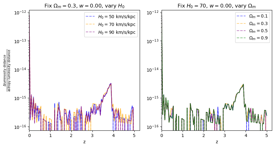
fractional_comparison("luminosity_distance");

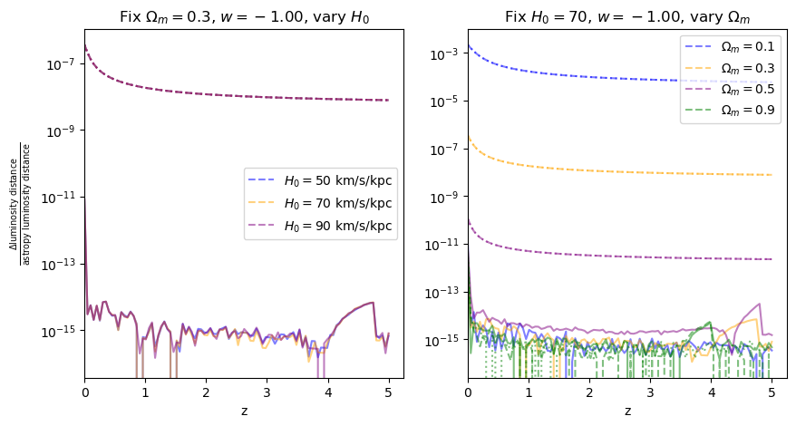
When \(\Omega_m=0.9\), the fractional error is comparable to floating point precision, which is why it looks a bit jaggedy.

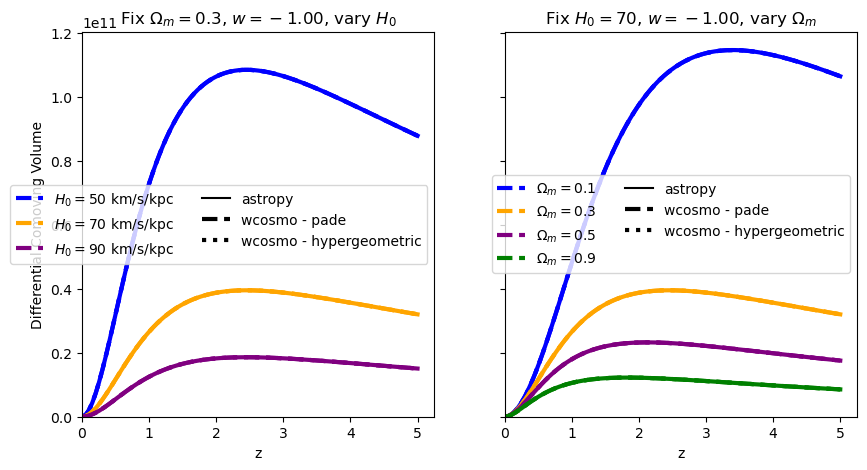
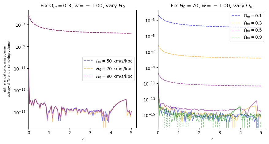
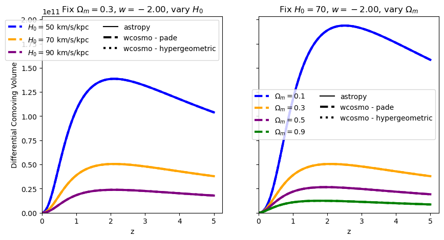
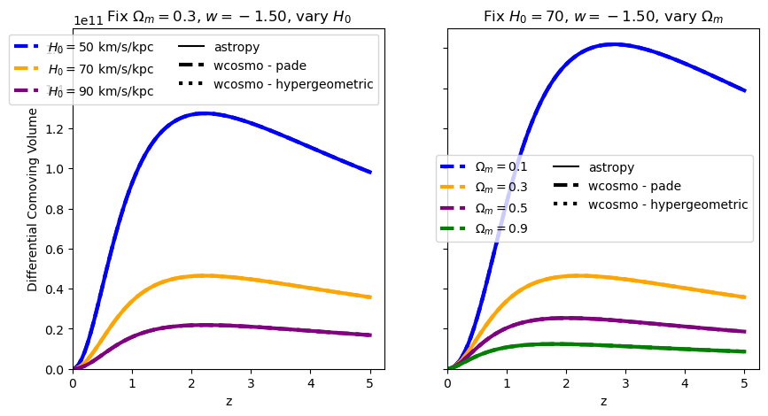
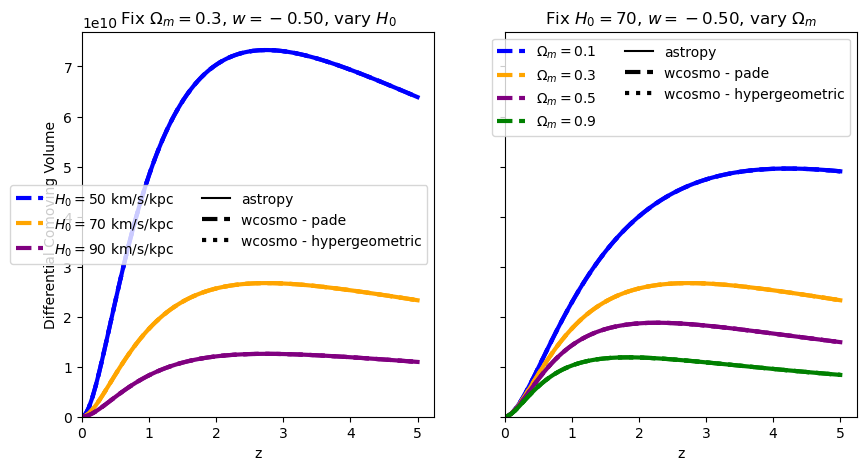
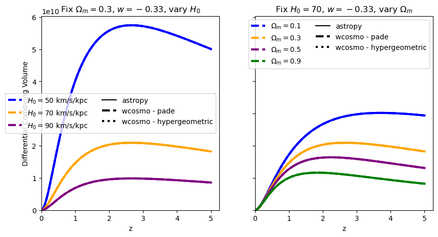
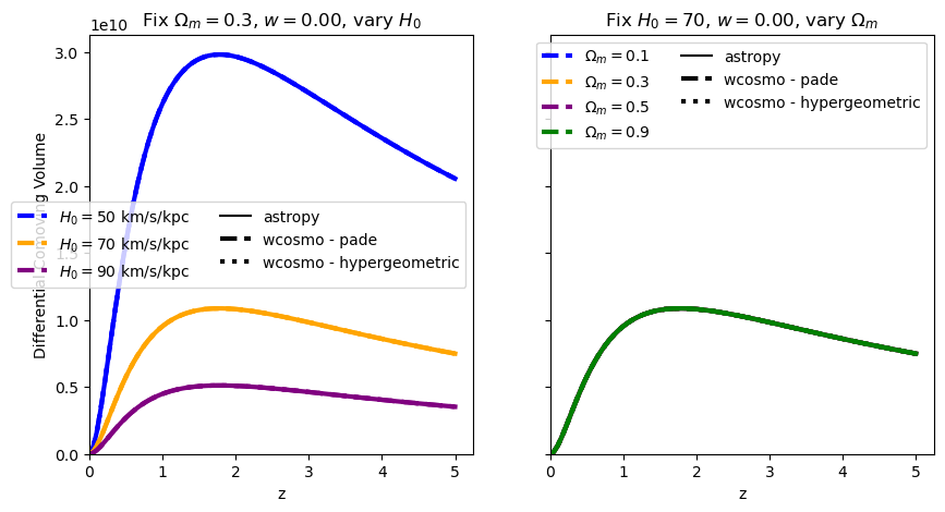
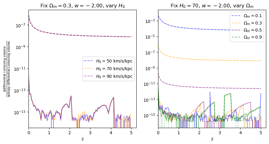
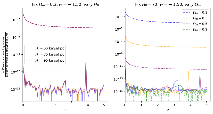
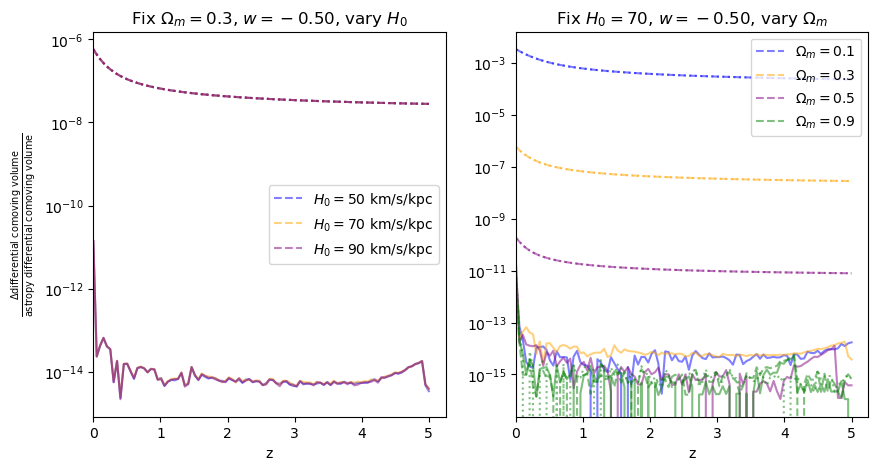
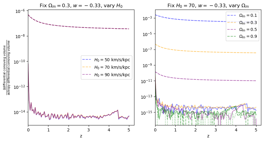
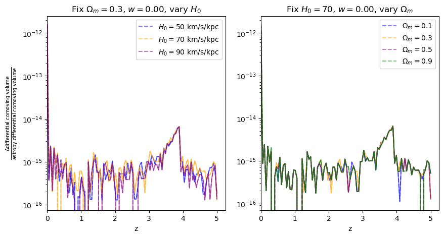
\(\frac{dV_c}{dz}\): differential comoving volume

absolute_comparison("differential_comoving_volume");

fractional_comparison("differential_comoving_volume");

\(\frac{d D_L}{dz}\): Jacobian between luminosity distance and redshift

Used commonly in GW data analysis

def dDL_dz(astropycosmo, z):
    dL = astropycosmo.luminosity_distance(z).value
    Ez_i = astropycosmo.inv_efunc(z)
    D_H = (Clight / 1e3) / astropycosmo.H0.value
    return np.abs(dL / (1.0 + z) + (1.0 + z) * D_H * Ez_i)


fig, axes = plt.subplots(nrows=1, ncols=2, sharex=True, sharey=True, figsize=(10, 5))
# axis 0: vary H0
axes[0].set_title("Fix $\Omega_m=0.3$, $w=-1$, vary $H_0$")
for H0, c in zip(H0_vals, colors):
    axes[0].plot(
        z_arr, wcosmo.FlatLambdaCDM(H0=H0, Om0=0.3).dDLdz(z_arr), ls="--", lw=3, c=c
    )
    axes[0].plot(
        z_arr,
        dDL_dz(FlatwCDM(H0=H0, Om0=0.3), z_arr),
        c=c,
        label=f"$H_0=${H0} km/s/kpc",
    )
axes[0].plot([], c="k", label="astropy")
axes[0].plot([], c="k", ls="--", lw=3, label="wcosmo")
axes[0].legend(ncol=2)

# axis 1: vary Om0
axes[1].set_title("Fix $H_0=70$, $w=-1$, vary $\Omega_m$")
for Om, c in zip(Om_vals, colors):
    axes[1].plot(
        z_arr, wcosmo.FlatLambdaCDM(H0=70, Om0=Om).dDLdz(z_arr), ls="--", lw=3, c=c
    )
    axes[1].plot(
        z_arr, dDL_dz(FlatwCDM(H0=70, Om0=Om), z_arr), c=c, label=f"$\Omega_m=${Om}"
    )
axes[1].plot([], c="k", label="astropy")
axes[1].plot([], c="k", ls="--", lw=3, label="wcosmo")
axes[1].legend(ncol=2)

for i in [0, 1]:
    axes[i].set_xlabel("z")
    axes[i].set_xlim(left=0)
axes[0].set_ylabel("$\\frac{dD_L}{dz} [Mpc]$")

Text(0, 0.5, '$\\frac{dD_L}{dz} [Mpc]$')

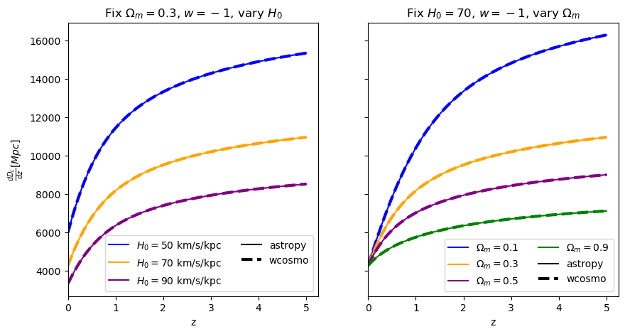
We find that the relative error is just a function of \(\Omega_m\) and redshift, not \(H_0\), which is expected as the approximant only changes \(D_L(z)\), leaving \(H_0\) as a constant factor common to both wcosmo and astropy’s calculations.

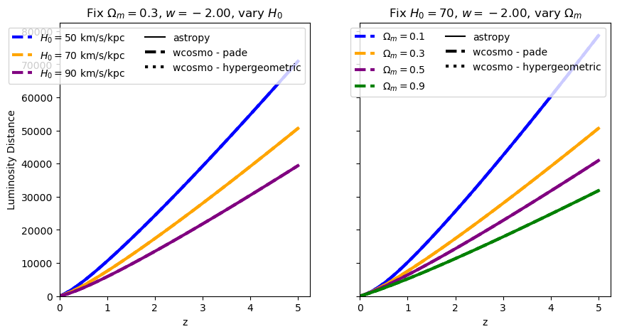
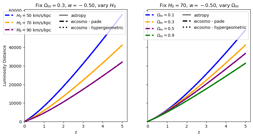
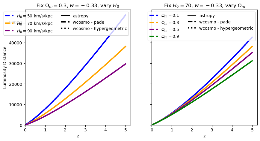
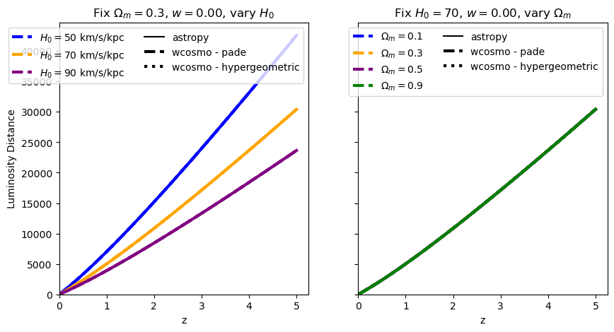
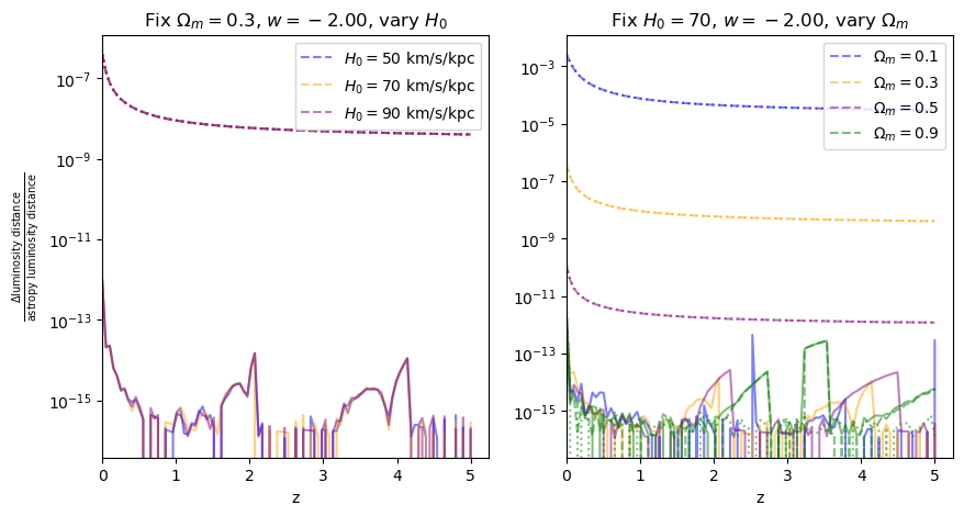
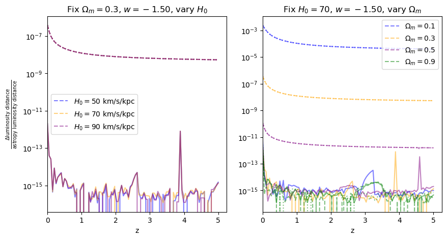
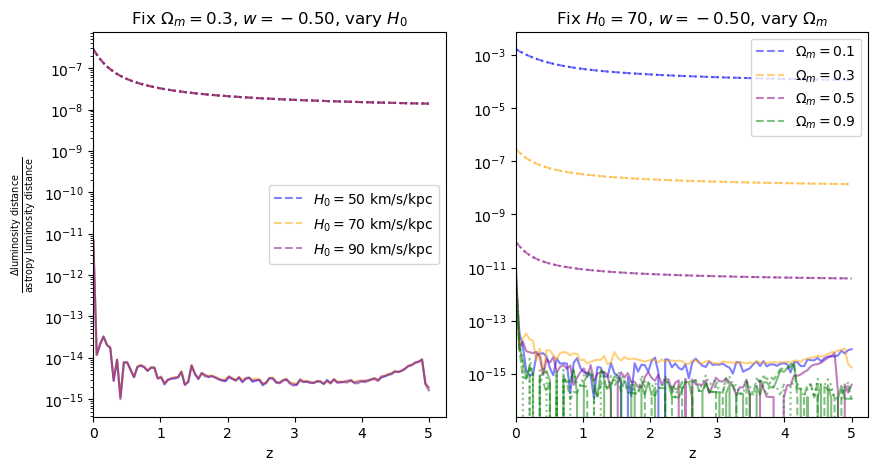
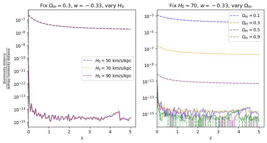
\(w\neq-1\)

This is where wcosmo differs from A&K2011. Let’s compare what we get with astropy, for various values of \(w\).

Luminosity distance

for w in w_vals:
    absolute_comparison("luminosity_distance", w=w)

for w in w_vals:
    fractional_comparison("luminosity_distance", w=w)

\(\frac{dV_c}{dz}\): differential comoving volume

for w in w_vals:
    f = absolute_comparison("differential_comoving_volume", w=w)
for w in w_vals:
    f = fractional_comparison("differential_comoving_volume", w=w)